Working with plate velocities in GPlates

GPlates v1.3 can display and extract plate velocities. Depending on your work, you might have different requirements for these domains, plus there are a few pitfalls on the way. Currently, there are two three  ways to create velocity domains in GPlates:

1. Create a global set of points at regular spacing which stay fixed absolute and the plates move across them. This method will report velocities of whatever plate will be on top of these points. This method is generally used when working with global models and when one wants to export boundary conditions for global geodynamic modelling (the CitcomS and Terra mesh generation options). Use Features → Generate Velocity Point Domains to create a velocity domain setup according to your needs. Note that this also allows to create a regular spaced lon/lat grid of distributed points. The features are gpml:MeshNode features in the GPlates Geological Information Model.
2. Alternatively, you can just go and create a set of points wherever you require them - you might have a few small plates which fall through the cracks when creating the global velocity domains. So here, you just go and create a few point features, assigning them the right properties in the 'Create Feature' dialogue. Create and save the layer after you are done. You can automatically assign PlateIDs using GPlates' cookie-cutting tool afterwards which saves you typing in PlateIDs manually.
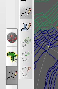
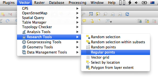
3. Use QGIS and the Vector toolbox to create a regular spaced point grid in OGR Vector format (ESRI Shapefile, OGR GMT etc) and load that into GPlates, cookie-cut - or rather - assign plate ids and there is a regional, regular-spaced point set which you can use as velocity domains.

One important thing to know is that GPlates utilises layers for different types of data, so here's a little digression and some background info. This layer business is much like GIS software has vector and raster layers, and other layers which are the result of some computations/combination of other layers - or like image manipulation applications like GIMP or Photoshop. The following layer types exist in GPlates (n.b. ideally a detailed overview of the layers with examples should follow here but currently there is no time, I suppose this might be found in the GPlates documentation somewhere):

• ReconstructionTree: Rotation files/models are automagically assigned to the yellow layer.
• ReconstructedGeometries: Essentially all feature data one works with gets stuffed into the green layer type. Shapefiles, standard GPML files (not topologies), OGR GMT files all belong to this layer type.
• Co-registration: Features related to data mining and association checks are combined in this layer type. This is one example where a layer does not correspond directly to a feature collection (ie a single file on disk). Instead, the user selects a set of seed points (a feature collection) and target geometries/rasters (another feature collection/raster) to generate a new data type.
• Calculated velocity fields: Another one of of those layers where the layer=feature collection equation breaks down. Here we load a point feature collection and combine it with other data such as topological polygons or static polygons to compute velocities.
• Resolved topologial networks:   This (brown) layer type is similar to the topological geometries but creates triangulated networks used for deformation.
• Resolved topological geometries: Topologically closed polygons are created from the combination of a rotation file (ReconstructionTree) and a feature layer (ReconstructedGeometries).
• Reconstructed Raster: Raster data gets loaded into the red layer type.
• 3D scalar field: Volume-rendering of scalar fields as, for example, from seismic tomography

Now that this is sorted, let's generate some velocity fields.

After completing either of those steps above you should have a point layer from which you can now extract velocities. Depending on the way you created these points, the steps to display velocities might differ a bit.

1. Create a global velocity domain layer using (1) from above or create your velocity points using method 2 or 3 from above.
2. Once you have created the velocity domain layer using option (1), GPlates will automatically load a new feature layer with the name of velocity point layer as you specified. If you have  used the “Latitude Longitude” option in GPlates, your default layer name will be something like lat_lon_velocity_domain_SomeIntegervalue and have a green color in the layer window (the ReconstructedGeometry layer). In addition, GPlates will create a aqua turquoise colored layer (the “Calculated Velocity Fields” layer) with the same name. That is where the action happens.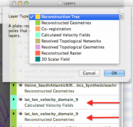
3. The next thing you need is either a static polygon feature collection set or a topologically closed polygon feature collection and of course a rotation model loaded. The next steps will illustrate why.
4. Only if you have created your point velocity domain layer manually): Add a new blank “Calculated Velocity Fields” layer throug clicking the big + at the top of the layer window.
5. The key now is to connect the Velocity layer with other feature data. This can be a global polygon data set or a set of static polygons. Open the aqua-colored layer by clicking the little triangle on the left and  under the “Inputs” category you see the headings “Velocity domains” (and your generated velocity domain reconstructable geometry layer is already connected to this. If it is not connected, you need to add it here. This is  the case where you created it manually. Under the “Velocity surfaces” heading, click on the “Add new connection”  field and select the polygon data. If one is set to export velocity boundary conditions for geodynamic modelling this of course requires continuously closed polygons, covering the surface of the Earth at any reconstruction time. Such topologically closed polygon data is provided on the EarthByte website. If you are working regionally, just select whatever polygon feature collection you are working with.
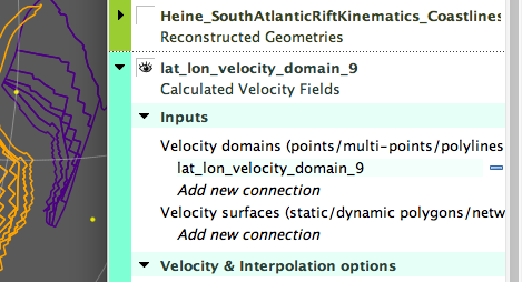
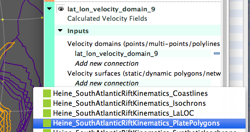
6. In the case that you are using global velocity domain points and polygons, make sure that in the “Velocity and Interpolation options” section,  Calculate velocities is set to “of surfaces” . If you have a set of points that are assigned plate ids, one would want to set this to “of domain points”.
7. Once you have connected your surface domains with your velocity domains, you should see velocity vectors displayed in the main window. The settings for the vector display can be altered in the layer dialogue.
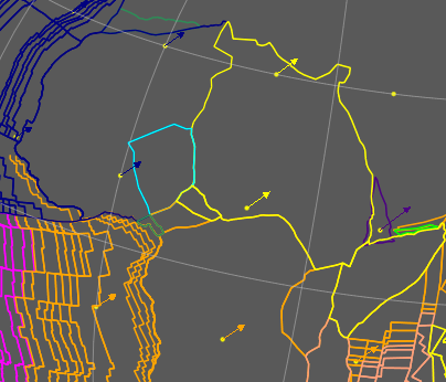
8. If needed these vectors can be exported using the Export… function under the Reconstruction menu in a wide flavour of formats.